This guide starts at the application's Start Center and follows the sequence: create a model, configure inputs, run the simulation, inspect results, then save and export. For a first run, keep the defaults to produce an example you can compare with the documented results.
1. Choose a starting point
| Start Center action | Purpose |
|---|---|
| New Model | Create a project or run the default example |
| Open Project | Continue editing an existing project |
| Open Result / Package | Inspect saved results or exported content |
Opening, recovering, or converting a project does not run a calculation automatically. A read-only result is for inspection; open an editable project to change inputs.
2. Create a model with default options
Click New Model, keep the following choices, and click Finish.
| Wizard option | Default selection |
|---|---|
| Model family | Empirical Frequency Lifetime Solver |
| Solver domain | Frequency statistical |
| Thermal / Pack | Average thermal table |
| Temperature source | Manual / default daily max-min |
Check the main example conditions: battery energy of 423 kWh, range of 235 km, weekly distance of 1,400 km, 365 operating days per year, 180 months, and Wuhan daily temperatures. The example uses the default sequential mode: cycle aging first, then calendar aging.
These data illustrate the workflow. Create or save a separate project and replace them with suitable cell and operating data for an actual assessment.
3. Configure and review inputs
| Order | Input area | Main checks |
|---|---|---|
| 1 | Cell page: vehicle and lifetime parameters | Total and usable battery energy, range, cycle/calendar lifetime data, temperature anchors, and degradation parameters |
| 2 | Pack | Pack configuration, thermal management, and temperature-rise assumptions |
| 3 | Operating conditions | Daily mileage, energy and charging shares; weekly driving, parking, fast/normal charging periods, and SOC |
| 4 | Temperature | Daily maximum/minimum values, units, missing data, and source; maximum must not be below minimum |
| 5 | Cell page: run settings | Operating days per year, total months, target years/mileages, and iteration mode |
Follow the units shown in the interface. Distinguish fractions from percentages and pack energy in kWh from cell capacity units. Retain data sources and processing notes alongside the values.
Some packaged daily-temperature application paths in the Temperature Data Center use estimated series and have a known source-labeling issue. Verify the daily temperatures applied to the project. A source label alone does not establish that a series contains original measurements. Referencing minute- or second-resolution data also does not mean the lifetime solver uses that time step.
The screenshots below show the current software build running locally in a browser, with the default inputs of a new model before simulation. Click an image to view it at its original size. Values displayed as -- have not yet been calculated; screenshots retain the version identifier shown by the application.
3.1 Cell, vehicle, and run parameters
Location: Model Inputs → Cell. This page defines the cell degradation basis, vehicle energy conditions, and simulation duration. Select an applicable degradation basis, then review the lifetime parameters and operating conditions.
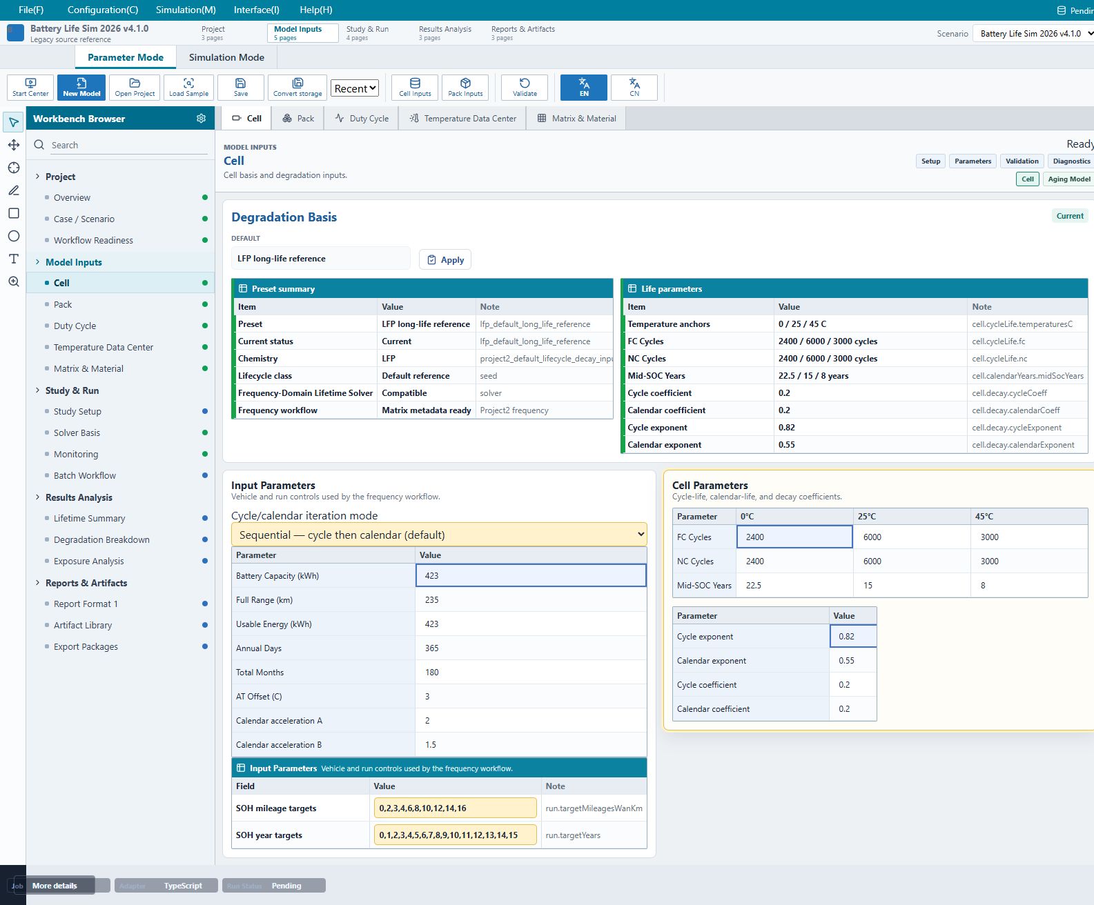
| Parameter group | Meaning and entry guidance |
|---|---|
| Battery energy and range | Enter battery capacity and usable energy in kWh, and full-charge range in km. Defaults are 423, 423, and 235 respectively. Do not enter an Ah capacity directly into an energy field. |
| Assessment period | Annual operating days and total months define the assessment period: 365 days and 180 months by default. Target years and mileages define result queries; mileage inputs use units of 10,000 km. |
| Lifetime temperature anchors | Enter fast-charge cycle life, normal-charge cycle life, and mid-SOC calendar life at 0, 25, and 45 °C. Cycle life is in cycles; calendar life is in years. |
| Degradation parameters | Cycle/calendar exponents, coefficients, and calendar acceleration parameters belong to the selected empirical model. Keep them consistent with the test conditions and calibration basis of the lifetime data. |
| Temperature offset and iteration mode | Review the temperature-offset assumption and the update order for cycle and calendar loss. Keep these consistent between comparisons or document changes. |
The default LFP reference data illustrate the workflow. When changing the cell, review temperature, SOC, charging conditions, and end-of-life criteria rather than retaining all lifetime parameters after changing only the material name.
3.2 Pack and thermal management
Location: Model Inputs → Pack. This page records pack configuration and provides the temperature-rise conditions used by the frequency-domain calculation.
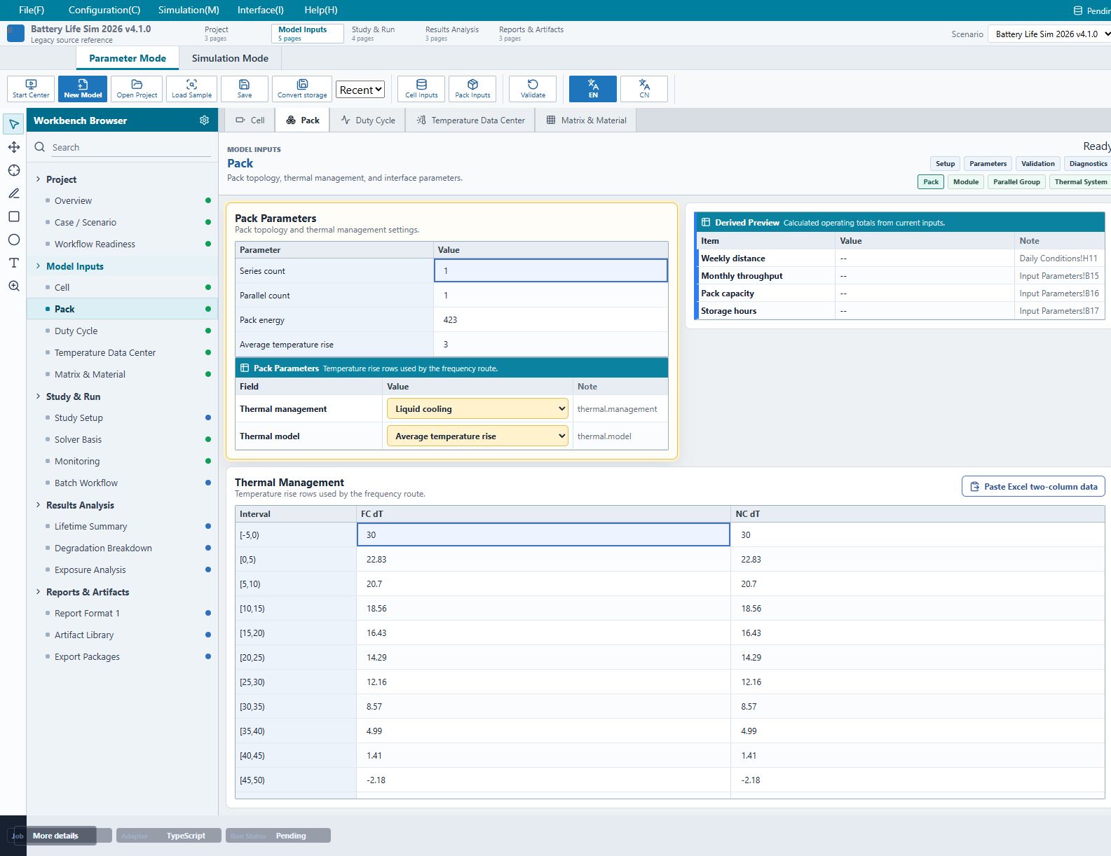
| Parameter group | Meaning and entry guidance |
|---|---|
| Pack parameters | Series count, parallel count, and pack energy describe the project configuration. Check consistency with vehicle energy conditions. Their presence in the interface does not establish support for a complete electrical-network analysis. |
| Thermal management and model | Record the management method, such as liquid or air cooling. The default route uses average temperature rise/thermal tables; 0D and 1D options marked Reserved are not currently available thermal models. |
| Temperature-rise table | Enter fast-charge FC and normal-charge NC temperature differences, dT in °C, for each ambient-temperature interval. Two-column pasting is available. These are differences relative to ambient temperature, not absolute cell temperatures. |
| Derived preview | Weekly distance, monthly energy throughput, and related values are calculated, not entered manually. Check their consistency with the duty cycle after running. |
Use temperature-rise data from applicable pack tests, thermal simulations, or documented engineering assumptions. This page does not solve a spatial temperature field.
3.3 Daily conditions and weekly states
Location: Model Inputs → Duty Cycle. Daily Conditions defines energy and distance; Weekly States defines driving, parking, and charging schedules. Together they describe a repeating operating week.
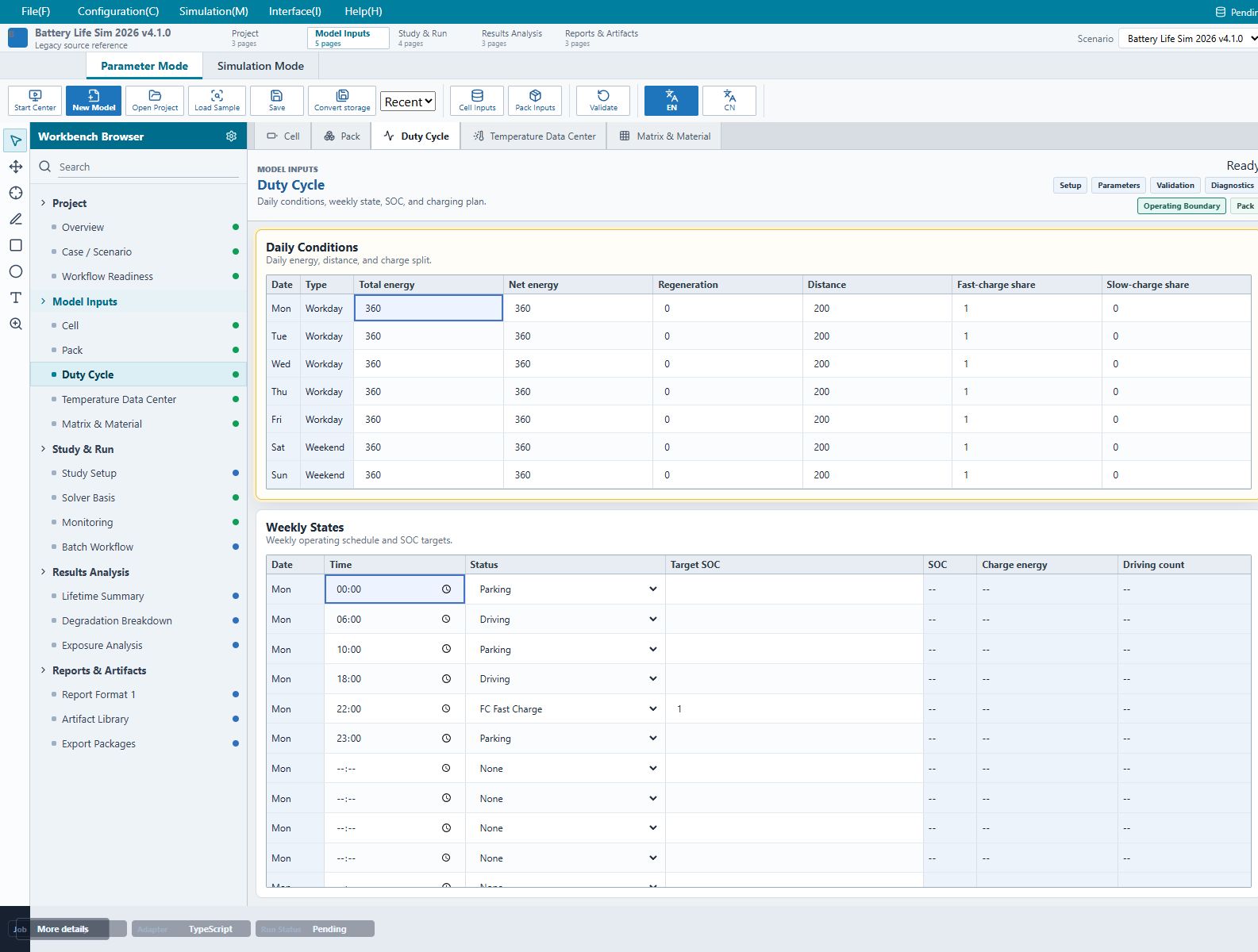
| Input area | Meaning and entry guidance |
|---|---|
| Daily conditions | Enter total, net, and recovered energy in kWh and distance in km for each day. Defaults are 360 kWh total and net energy, zero recovered energy, and 200 km per day. |
| Charging shares | Fast- and normal-charge shares use fractions from 0 to 1; 1 means 100%. Check consistency with the intended charging strategy. |
| Weekly states | Configure parking, driving, DC fast charging, and AC normal charging in chronological order. Fill only the events in use; unused rows may remain empty. |
| Target SOC | Charging targets use fractions from 0 to 1: enter 0.8 for 80%, not 80. |
| Calculated columns | SOC, charging energy, and trip count are derived values. The -- placeholders update when the corresponding results are calculated. |
Check event order and consistency between driving schedules and daily energy. After running, inspect the weekly operating profile to review SOC and charging behavior.
3.4 Temperature sources and daily values
Location: Model Inputs → Temperature Data Center. Current summarizes the active project conditions, Library provides selectable references, and Import exposes project weather editing and pasting.
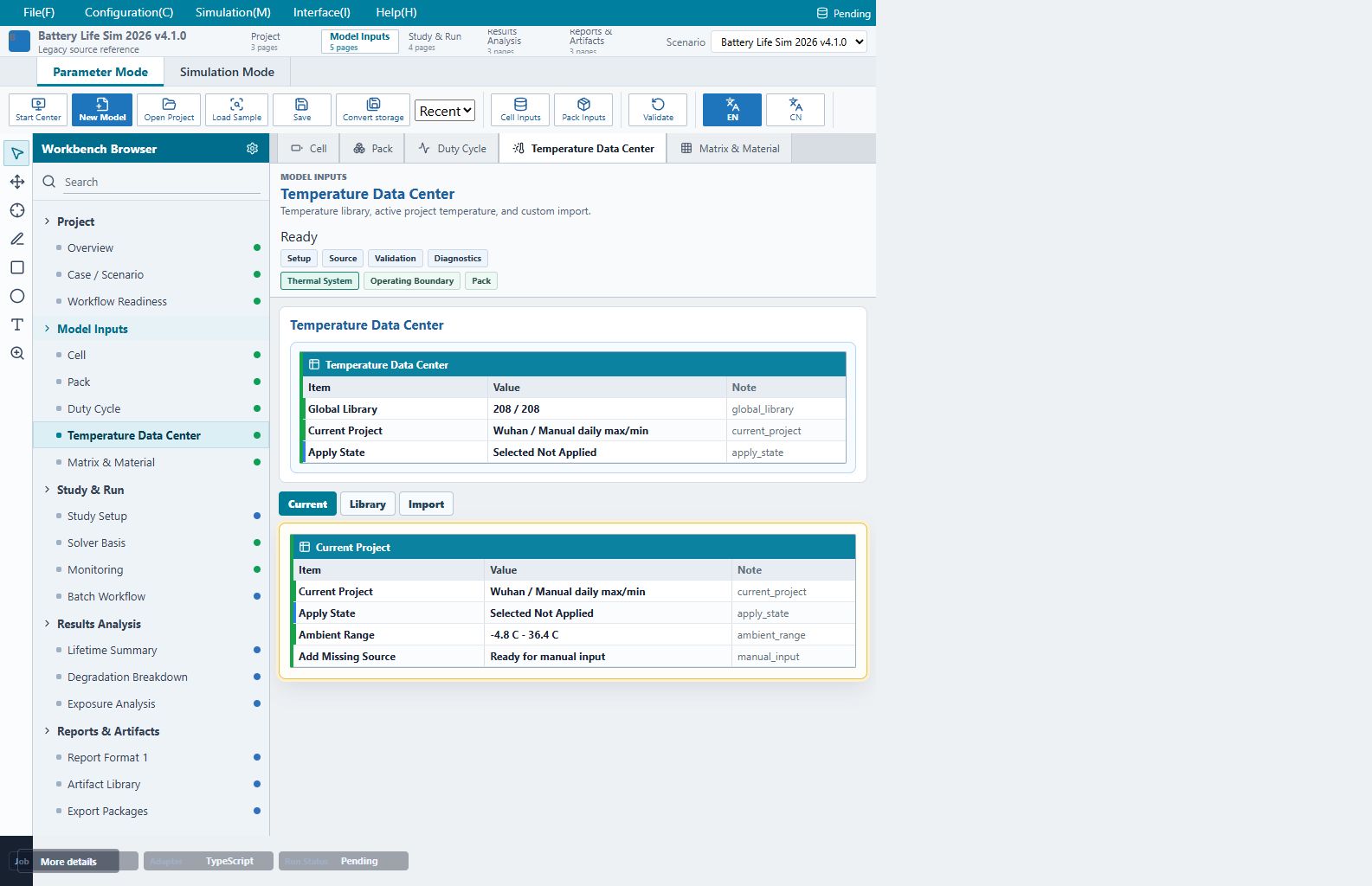
The default project uses 365 days of daily maximum/minimum temperatures for Wuhan, spanning approximately −4.8 to 36.4 °C. Selected Not Applied describes the selection state of a library entry; use Current Project and the actual daily table to identify the data in use.
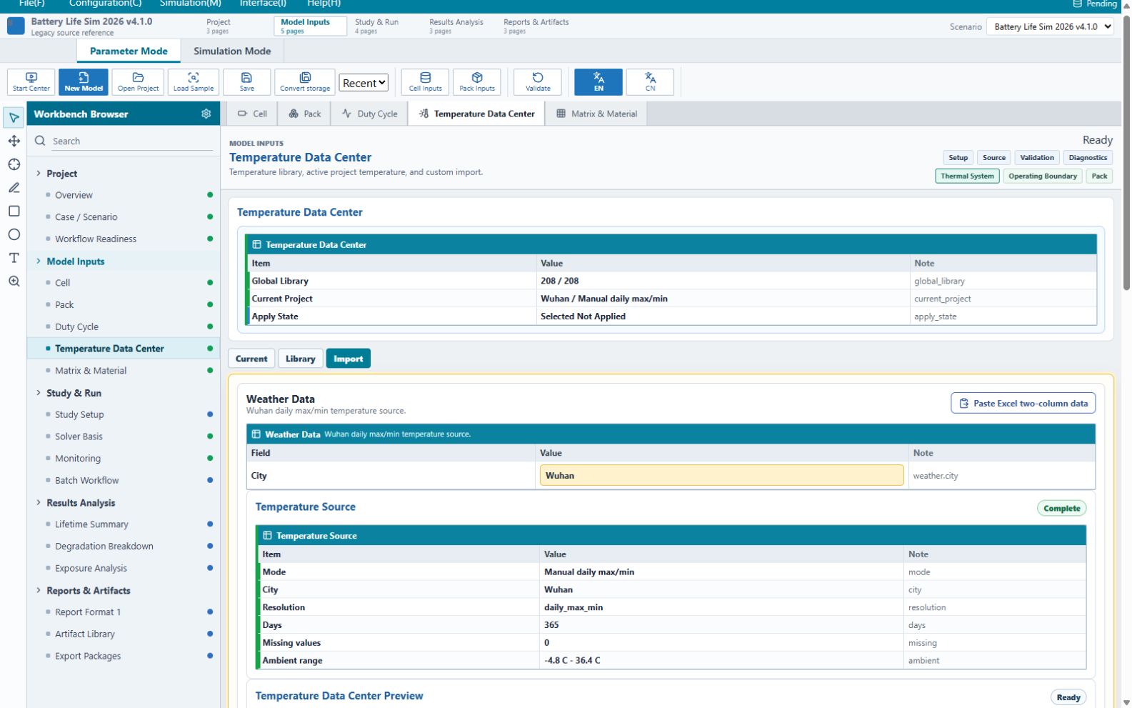
| Action | Entry and review guidance |
|---|---|
| Prepare daily temperatures | Arrange daily maximum and minimum temperatures in two columns in date order, in °C. Check the year, day count, missing cells, and rows where maximum is below minimum. |
| Enter data | Edit the table on Import or use Paste Excel two-column data. Excel import is currently marked Reserved; this does not indicate support for importing workbook files directly. |
| Apply and review | When using Apply Project Weather, review the data and select Confirm update project weather first. Then check Current and the daily table. Changing the city label or selecting a library entry alone does not replace the entire temperature series. |
| Retain the source | Record source, year, and processing method. Preview examples on the page are distinct from active project data; use the project daily table for the assessment. |
3.5 Role of the Matrix & Material page
Location: Model Inputs → Matrix & Material. The current page displays weight factors and a decay matrix generated from calculation results. It is not a form for entering lifetime data cell by cell. Configure cell lifetime data on Cell; use this page after running to inspect temperature/SOC weights and intermediate degradation results. A new, uncalculated project does not require manual matrix entries here.
3.6 Iteration mode
- Sequential — cycle then calendar (default): calculate the monthly cycle increment first, then calculate the calendar increment using the updated total loss.
- Parallel inverse: calculate both increments using total loss at the beginning of the month.
The modes can produce different results. Record both algorithm version and iteration mode when comparing runs. Opening a historical project does not recalculate its retained results automatically.
4. Run the simulation
- Enter Simulation Mode and resolve blocking input-validation messages.
- Click Run Simulation.
- Review status and logs in the monitor and wait for completion.
- Open Results Analysis to inspect result status, final SOH, and curves.
The verified default example contains 181 curve points covering months 0–180 and ends at approximately 55.8965% SOH. Use this comparison only when inputs, algorithm, and iteration mode match. See Understanding results for the curves and their meaning.
Currently, Stop clears the displayed running state but may not terminate background computation. Do not repeatedly stop and immediately submit new tasks during a long calculation.
5. Check the operating profile and result source
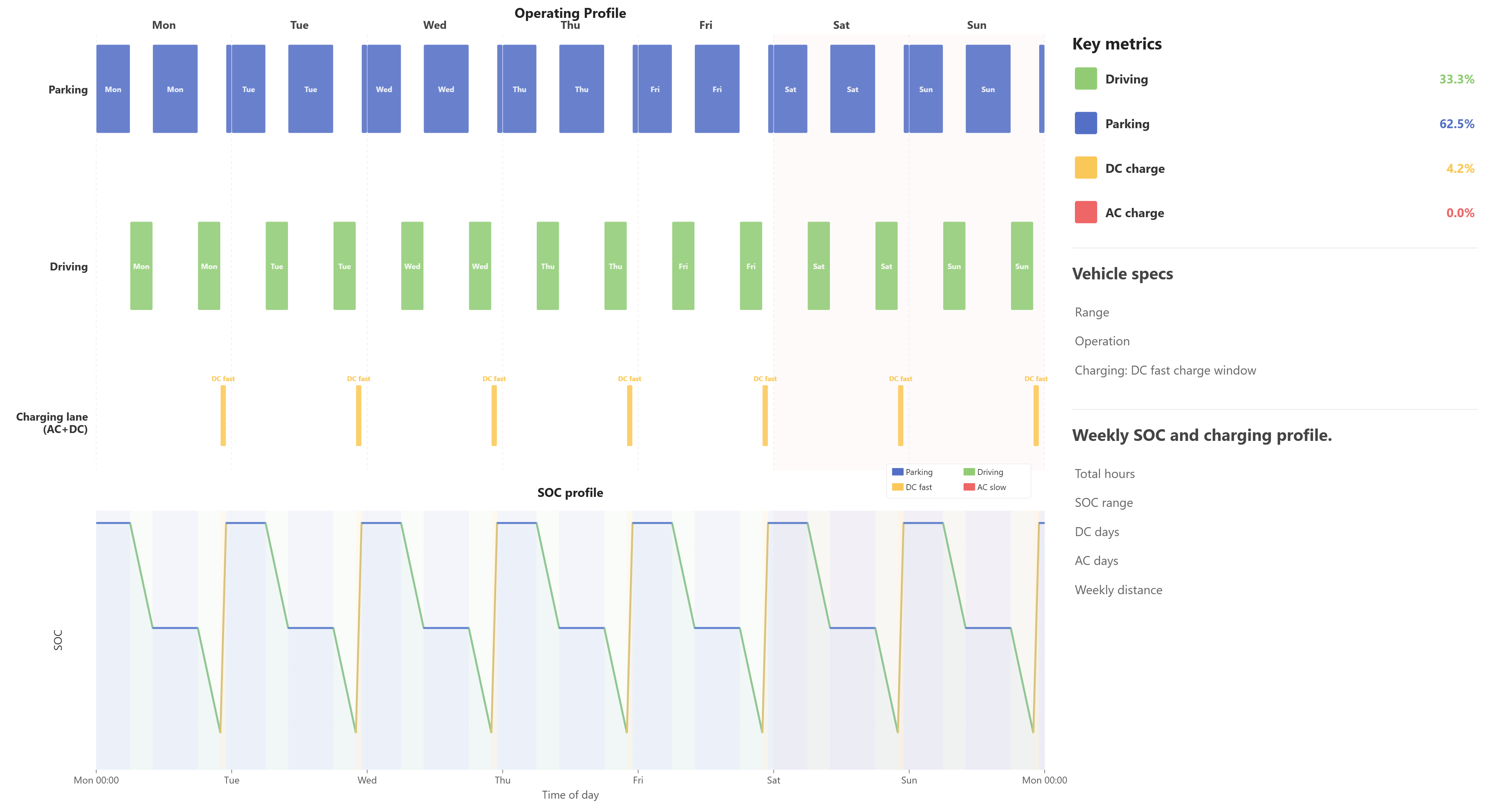
Figure: the weekly operating profile exported from the actual default run. Check driving and parking periods, charging schedules, and SOC before interpreting long-term lifetime results.
After inputs change, an older result no longer represents the new scenario. If export is disabled or marked stale, run again. Select the corresponding historical run explicitly when inspecting older results.
6. Save projects and results
Choose a storage format on the first save; subsequent saves use that format. Save again after generating reports to retain the latest report versions.
| Format | Purpose and handling |
|---|---|
.blsimproj with its _blsim_files directory |
Managed project; retain the entry file and companion directory when moving or backing up |
.blsim |
A single-file project containing editable project state |
.blsimresult |
A read-only document for inspecting a selected result |
Use Save As to preserve the original before a new assessment. HTML, PPTX, and CSV reading/data files do not replace a full project backup; they do not contain the complete editable state.
7. Prepare and export reports
Open Reports & Artifacts → Report Format 1 and enter the report name, date, author, reviewer, assessment background, model basis, and supplemental information. Verify default template text against the actual project.
Select a format in the toolbar and click Export Report.
| Format | Purpose |
|---|---|
| HTML | Read and review pages in a browser |
| PPTX | Present results; check fonts and layout after opening |
| Report package | Retain the report, figures, sampled tables, inputs, and indexes together |
| Export CSV | Generate a separate data package for numerical review |
Report-package tables may be sampled at intervals. Use the full solver results for monthly checks rather than treating three example rows or a sampled table as complete output. See Understanding results for field definitions and known discrepancies.
Common situations
| Symptom | Suggested action |
|---|---|
| Simulation cannot run | Check for a read-only session, an unsupported model selection, or blocking messages |
| Export is unavailable or stale | Check whether computation completed and whether inputs changed afterward |
| An older package exposes only some content | It may contain exports only; obtain the full project to continue editing |
| Results differ from the default example | Compare input snapshots, units, temperature sources, algorithm versions, and iteration modes |
| Charts and report tables differ | Check cumulative versus incremental quantities, time ranges, and axis conversions using the results guide |
Read the results guide · Return to the overview · Software contact
Documentation and example evidence: September 8, 2026. Frequency-domain Lifetime Simulation and the Battery Life Sim name in screenshots refer to the same workbench.
Back to top