First identify the inputs behind a result, then examine SOH and cycle/calendar losses, and finally check the conversions to time, energy throughput, and mileage. Multiple views describe different aspects of the same run.
Main quantities
| Quantity | Meaning and units |
|---|---|
| SOH | Model-predicted capacity retention, usually displayed as a percentage; a fraction of 1.0 corresponds to 100% |
| Total loss / Decay | Cumulative loss relative to initial capacity; 0.1 means a loss of 10% of initial capacity |
| Cyclic Loss | The contribution attributed to cycle aging by the model; distinguish cumulative values from per-iteration increments |
| Calendar Loss | The contribution attributed to calendar aging by the model; distinguish cumulative values from per-iteration increments |
| Time | Service duration, with 12 months per year |
| ETP | Cumulative energy throughput; values here use kWh, while chart axes may use scaled ticks |
| Mileage | Cumulative distance; values here use km, while chart axes may use scaled ticks |
For the cumulative results shown here: SOH (%) = (1 − total loss) × 100, and total loss = cumulative cyclic loss + cumulative calendar loss.
A cyclic loss of 0.212485 means approximately 21.2485 percentage points of initial capacity lost. It does not mean that cycle aging accounts for 21.2485% of total loss. Align fractions, percentages, and percentage points before comparing values.
Default example conditions
The following results come from the default example run and verified on September 8, 2026. Its algorithm ID is frequency_domain_lifetime_solver, algorithm version is 4.1.0, and iteration mode is sequential_cycle_then_calendar_v1.
| Condition | Value |
|---|---|
| Total / usable battery energy | 423 / 423 kWh |
| Driving range | 235 km |
| Weekly distance | 1,400 km |
| Operating days per year | 365 |
| Duration | 180 months, or 15 years |
| Temperature | Built-in Wuhan daily maximum/minimum temperatures, 365 days |
| Iteration order | Cycle aging first, then calendar aging |
Capacity retention over time
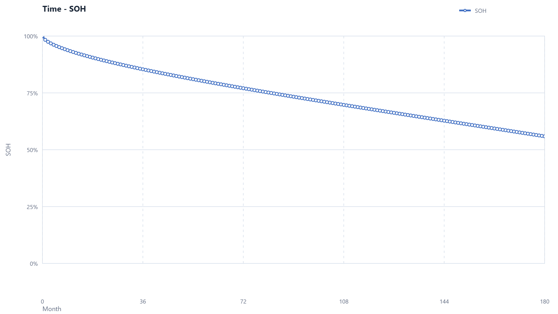
Figure: the time–SOH curve exported from the actual default run. It contains 181 points covering months 0–180. The table selects a few months for readability; both loss columns contain cumulative values.
| Month | SOH (%) | Cumulative cycle loss (pp) | Cumulative calendar loss (pp) | Cumulative energy (kWh) | Cumulative mileage (km) |
|---|---|---|---|---|---|
| 0 | 100.0000 | 0.0000 | 0.0000 | 0 | 0 |
| 12 | 92.6014 | 1.6951 | 5.7035 | 131,400 | 73,000 |
| 60 | 79.6646 | 7.0439 | 13.2915 | 657,000 | 365,000 |
| 120 | 67.3846 | 13.8145 | 18.8008 | 1,314,000 | 730,000 |
| 180 | 55.8965 | 21.2485 | 22.8550 | 1,971,000 | 1,095,000 |
Here, pp means percentage points of initial capacity. The unrounded final SOH is 55.896509917728444%. Displaying 55.90% in the interface or report is a rounding difference, not evidence of different calculations. Rounded components can also differ in the last digit when added; use raw values for precise checks.
Cycle and calendar losses
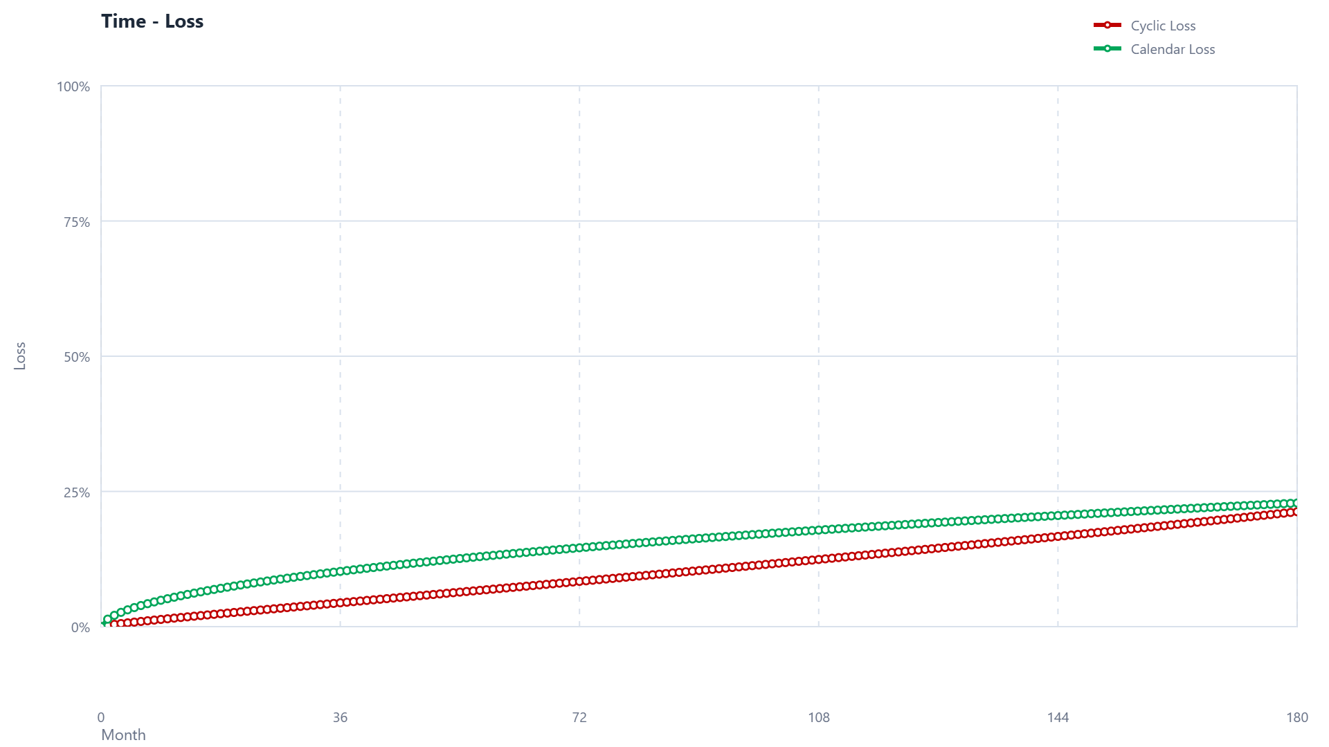
Figure: cumulative cycle and calendar losses from the default example. At month 180 they are approximately 21.2485 and 22.8550 percentage points, respectively, giving a total loss of approximately 44.1035 percentage points.
This breakdown depends on the model, input data, assumptions, and iteration rules. It is not a direct experimental measurement of the two mechanisms. Keep cell data, algorithm, and definitions consistent when comparing scenarios, and state which inputs changed.
Why there are three horizontal axes
Time, ETP, and mileage views use the same lifetime result series. The default example uses these postprocessing conversions:
- Monthly distance = weekly distance × operating days per year ÷ 7 ÷ 12, approximately 6,083.3333 km.
- Monthly energy throughput = 10,950 kWh, derived from the default operating-energy totals.
- Cumulative distance and energy equal their monthly values multiplied by elapsed months.
Month 180 therefore corresponds to 1,095,000 km and 1,971,000 kWh. These are conversions for this example's inputs, not universal lifetime or mileage guarantees.
Reading an exported report
| Pages | What to check |
|---|---|
| 00–01: cover and contents | Name, date, attribution, and completeness |
| 02–03: background and model | Assessment requirements, data sources, model basis, and assumptions |
| 04: input summary | Inputs belong to the run, with traceable algorithm and iteration mode |
| 05: result summary | Final SOH, cumulative losses, and the basis of the conclusion |
| 06: weekly profile | Driving, parking, charging, and SOC match the intended scenario |
| 07–09: time, ETP, mileage | Axes, units, sampled points, and loss definitions agree |
Replace default model descriptions, attribution placeholders, and statements such as “no deviation recorded” with accurate project information. Completing those fields does not verify their contents automatically.
Verified report discrepancies
The following issues occur in the original reports exported from the default example. The example table on this page uses the verified full postprocessing results; writing this explanation has not corrected the application's report template.
| Item | Current behavior | How to review it |
|---|---|---|
| ETP detail table | The final value is shown as 46.2 kWh, while cumulative throughput ends at 1,971,000 kWh | Different quantities are used; check cumulative throughput against the full postprocessed series |
| Mileage detail table | It ends at 1,092,000 km using 52 weeks per year; the curve ends at 1,095,000 km using 365 days per year | Use the actual operating-day basis consistently |
| Loss detail columns | Some tables show per-iteration increments, while the summary and plots show cumulative losses | Identify increments and cumulative values before comparing |
| PASS / REVIEW | Some conclusions use a fixed 70% SOH threshold despite referring to a configured threshold | This does not establish project warranty compliance; changing target text does not change the fixed check |
| Text and layout | Chinese mode still contains English text and missing translation markers; figures overlap titles on pages 06–09 | Inspect exported pages; also open PPTX files in presentation software |
Review numerical results, successful file generation, and engineering conclusions separately. The default example establishes a numerical reference for the current implementation, not cell-specific experimental calibration or formal warranty validation.
Information to retain
Keep the input snapshot, raw result, algorithm version, iteration mode, temperature source, and report settings and generation date. State whether a table contains the full monthly series or sampled rows; a few report example rows do not replace all iteration records.
After correcting inputs or report definitions, save a new result/report version and record why it changed. This distinguishes operating-condition changes, algorithm changes, and corrections to report presentation.
Return to the user guide · Return to the overview · Software contact
Documentation and example evidence: September 8, 2026. Frequency-domain Lifetime Simulation and the Battery Life Sim name in screenshots refer to the same workbench.
Back to top